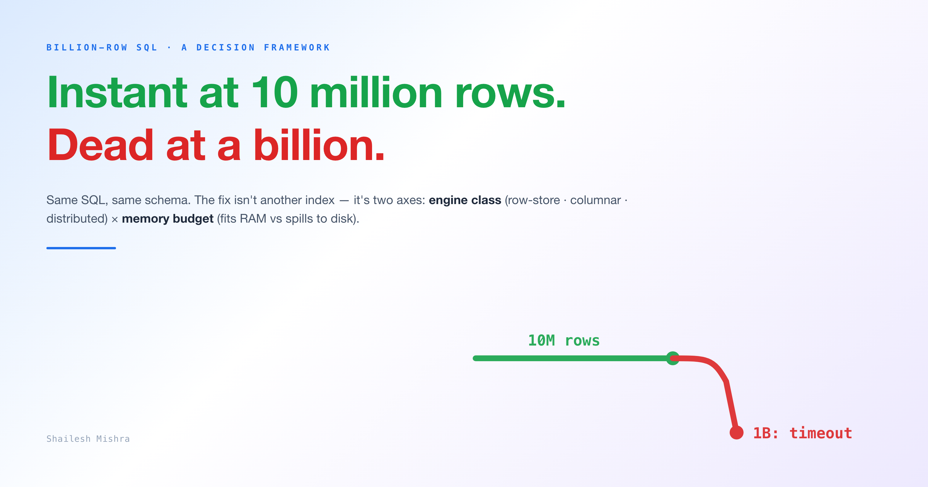
A query that returns in 40 milliseconds on ten million rows can time out completely on a billion. Same SQL, same schema, same database. I’ve watched a lot of teams hit that wall and go hunting for the one fix: a cleverer index, a bigger instance, whatever database was trending that month. There isn’t one fix. There are two questions that decide almost everything. What engine class is this workload on — row-store, columnar, or distributed? And does the query’s working set fit in memory, or does it spill to disk? Answer those honestly and most “billion-row problems” quietly resolve. Answer them wrong and no amount of tuning bails you out.
The query that was instant at 10 million rows and timed out at a billion
Here’s the shape of it. It’s a composite; I’ve seen it often enough that the specifics blur.
A team builds a dashboard on their main OLTP database. One query carries it: count distinct users, grouped by day, over a date range. Against a 10-million-row staging copy it comes back instantly, everyone signs off, ship it. Months later production crosses a billion rows — roughly the 1.1-billion-row scale in Mark Litwintschik’s cross-engine benchmarks — and the identical query simply stops returning. On-call adds an index; nothing. A composite index; nothing. A bigger instance; somehow slightly worse. “Throw it at Spark,” one person says. “Just use ClickHouse,” says another. Nobody can explain why either would help. That’s the real problem: everyone is arguing tactics with no framework for the decision.
The query didn’t regress. It’s doing exactly what it always did. What changed is that the workload crossed two lines at once — it outgrew the engine class that suited it at 10M, and its sorts and hashes stopped fitting in memory. Name those two lines and the mystery turns into a decision you can defend.
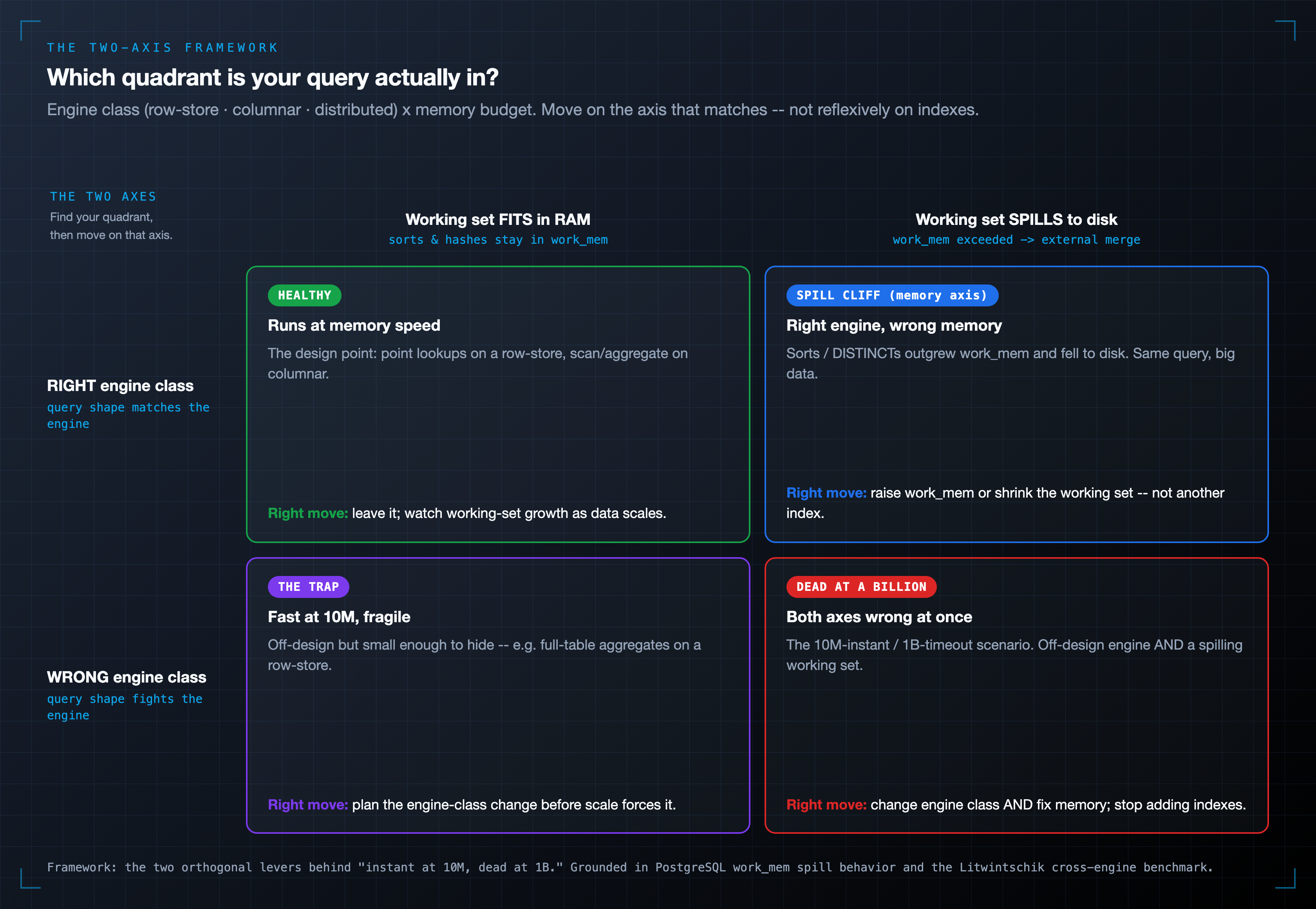
The two-axis framework
When a query dies at scale, the reflex is to index harder. Sometimes that’s right. At a billion rows it’s usually the wrong axis. Two levers actually decide whether a query survives.
Axis 1 — Engine class. Every database is built around one dominant access pattern, and that choice shapes everything downstream. A row-store OLTP engine (PostgreSQL, MySQL) keeps whole rows together and excels at “fetch or update this one record” and narrow ranges. A columnar/OLAP engine (ClickHouse, DuckDB, BigQuery) stores each column separately, so scanning and aggregating hundreds of millions of rows is the design point rather than the emergency. A distributed engine (Citus, Spark, Cassandra) spreads data across nodes for horizontal scale, trading query flexibility to get it. These are peers, not rungs on a ladder; none is “more advanced.” Run a workload on the wrong one and you get a query that flies at 10M and dies at 1B.
Axis 2 — Memory budget. Independent of engine class, every non-trivial query builds intermediate structures: sort buffers, hash tables for GROUP BY and DISTINCT, join tables. Fit those in RAM and the operation runs at memory speed. Overflow the memory the engine is allowed, and it spills to disk and falls off a cliff. PostgreSQL ships shared_buffers at 128MB and work_mem at just 4MB; the docs are explicit that a sort or hash exceeding work_mem starts “writing to temporary disk files” (PostgreSQL 18 — Resource Consumption, as of 2026). Four megabytes is nothing at a billion rows. This is the axis most write-ups skip, and it’s why the same query is fast one day and glacial the next. The SQL didn’t change; the data just got big enough to spill.
The axes are orthogonal. You can pick the right engine class and still hit the memory cliff, or keep memory in check and still be on an engine that’s wrong for the query’s shape. So the move is: work out which quadrant you’re actually in, then act on the axis that matches — change engine class, or change the memory budget — instead of adding another index to the axis that was never the problem.
Engine class 1: Row-store OLTP — great at point lookups, brutal on full-table aggregates
Row-stores are the workhorse for good reason. Ask for “order #48213 and its line items” or “the last 50 events for this user” and a row-store with the right index is hard to beat: it seeks to a handful of rows and returns. At 10M rows, the dashboard query was riding on that.
Aggregates over the whole table are a different story, and the reason is baked into how MVCC row-stores stay correct under concurrency. Because different transactions can see different versions of a row, the engine keeps no cached count of how many rows a table has. An exact count(*) therefore has to visit rows and check visibility — a sequential scan that grows linearly with the table.
The numbers are blunt. In Joe Nelson’s Citus benchmark on counting (PostgreSQL 9.5.4, 2016 — treat the milliseconds as illustrative of the mechanism, which is unchanged today, not as current figures), an exact count(*) ran 85ms at 1M rows, 161ms at 2M, and 343ms at 4M: a straight line, with the scan about 88% of the cost. Extend that to a billion rows and a single count is tens of seconds before any filtering. count(1) doesn’t rescue you; it measured slightly slower (99ms vs 85ms at 1M), because Postgres special-cases the argument-free count(*) while count(1) re-checks the argument on every row. And this isn’t Postgres being difficult — MySQL’s InnoDB shares the MVCC property and also has no O(1) table count.
When you don’t need an exact number, stop asking for one. Every row-store keeps a maintained estimate for its planner, and you can read it directly. In PostgreSQL that’s pg_class.reltuples (the Count-estimate pattern: SELECT reltuples::bigint FROM pg_class WHERE oid = 'schema.table'::regclass). In the same benchmark the estimate returned in about 0.3ms against 85ms for the exact count at 1M rows — roughly 280× faster, and effectively constant time at any size. The catch is accuracy: it’s an estimate and can’t apply a WHERE or DISTINCT. For “roughly how many rows” on a dashboard, that’s the difference between a billion-row scan and reading one catalog row.
None of this means “Postgres is slow.” It means a full-table aggregate is off-design for a row-store. Approximate counts, materialized rollups, and summary tables all soften it. But if scans and aggregates are your dominant pattern, you’re fighting the engine class — and that’s your first crossover signal.
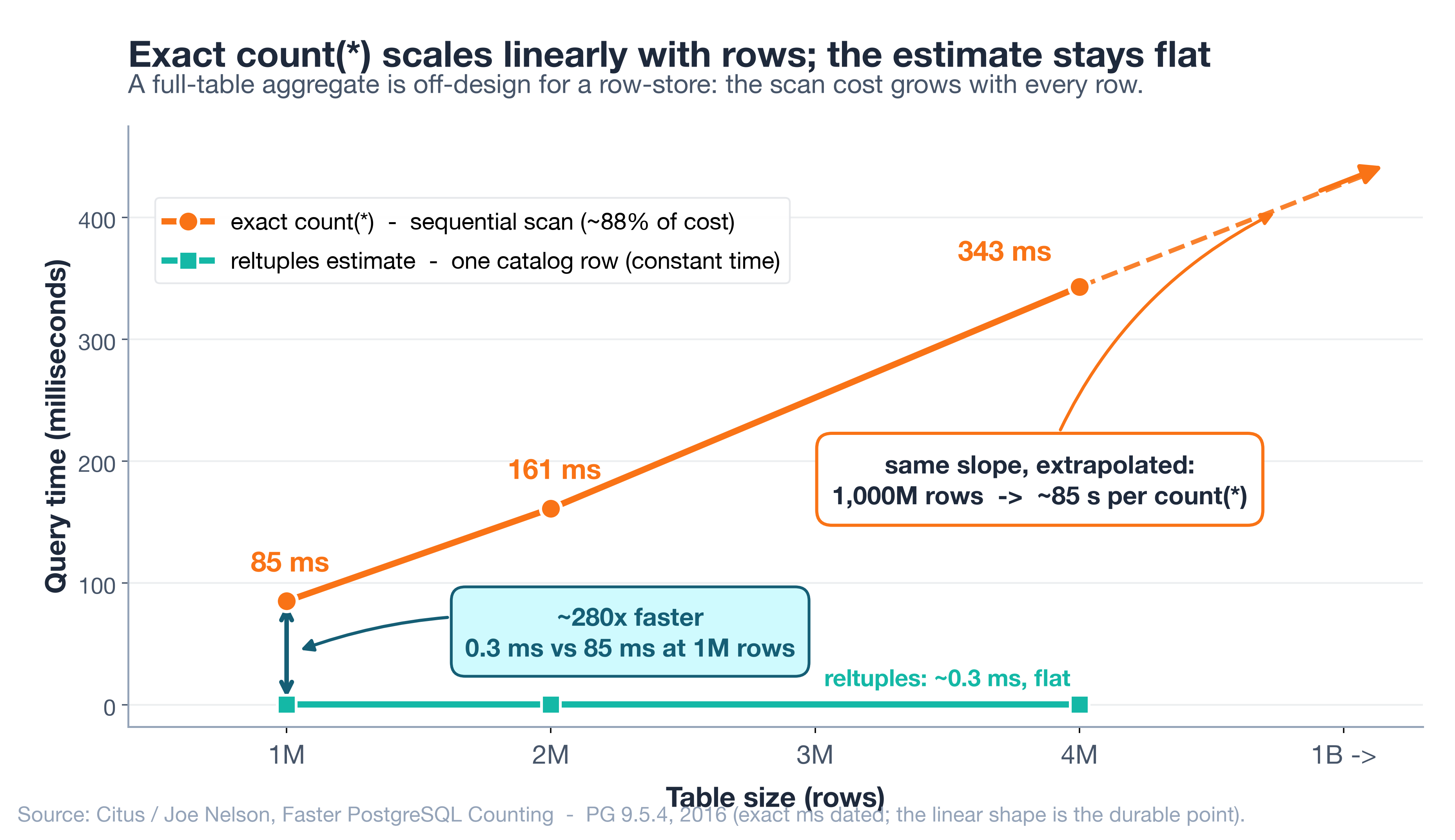
Exact count(*) vs the reltuples estimate. Source: Citus / Joe Nelson, PostgreSQL 9.5.4, 2016 — illustrative of the mechanism, not current figures.
Engine class 2: Columnar / OLAP — where scans and aggregates are the design point
If aggregates are killing your row-store, what’s built for them, and how much faster is it really? This is where the framework gets counter-intuitive.
Columnar engines store each column contiguously instead of packing whole rows. A scan-and-aggregate query that touches 3 of 51 columns reads only those 3 off disk; the other 48 are never opened. And because a column holds one type with heavy repetition, it compresses hard, so there’s less to read to begin with. Column pruning plus compression is why “scan a billion rows and aggregate” is routine here instead of an incident.
The headline number: Litwintschik’s 1.1-billion-row taxi benchmark (1.1B rows, 51 columns, ~500GB uncompressed; page updated March 2024) runs one analytical query across dozens of engines. On Query 1, a single desktop ran ClickHouse in 0.088s and DuckDB in 0.498s. The same query took 2.36s on a 21-node Spark cluster, 3.54s on 21-node Presto, and 1–3s on BigQuery. Postgres with the cstore_fdw columnar extension took 152–368s across the four queries, and plain SQLite’s format took 31,193s on Query 1 — about 8.7 hours, included to show what the wrong engine class actually costs.
A single desktop beat a 21-node cluster on a 1.1-billion-row scan by more than an order of magnitude. That one result is the whole framework in miniature. It isn’t that ClickHouse or DuckDB is “the best database” — it’s that for a scan-aggregate workload a columnar engine is in the right quadrant while the cluster pays coordination overhead it doesn’t need at this size. (Caveats: one benchmark, one hardware generation, recent desktop CPUs for the fastest single-node runs. Trust the shape of the gap, not the exact milliseconds.)
Compression is the other half, and it’s an economics lever as much as a speed one. ClickBench — the ClickHouse team’s scan/aggregate benchmark across 60+ systems — publishes a live “Data Size” column so you can compare on-disk footprint on the same ~100M-row dataset. Columnar layouts routinely pack this kind of wide, repetitive data down by a large multiple versus a row-store, though the exact ratio moves with engine, codec, and data, so read the live figure for the systems you’re weighing rather than trusting a headline number. (ClickBench is ClickHouse-run, so treat it as a scan-workload reference, not a neutral verdict.)
The honest counter-point: the same columnar engine that crushes the scan is the wrong tool for high-QPS single-row writes and point lookups. Insert a row and you touch every column store; update a field and compression works against you. The wide-column and key-value stores built for that job — Cassandra, ScyllaDB — sit at the opposite pole: excellent at point reads and writes on a known partition key, and structurally unfit for ad-hoc full-table aggregates. Cassandra’s CQL docs say it plainly: CQL “only allows select queries that don’t involve a full scan of all partitions,” and forcing one needs ALLOW FILTERING, whose performance the docs call “unpredictable.” A store modeled query-first around the partition key isn’t a scan-aggregate engine, which is exactly why ClickBench lists Cassandra and ScyllaDB among the systems it couldn’t benchmark on that suite. Right engine, wrong job, in both directions.
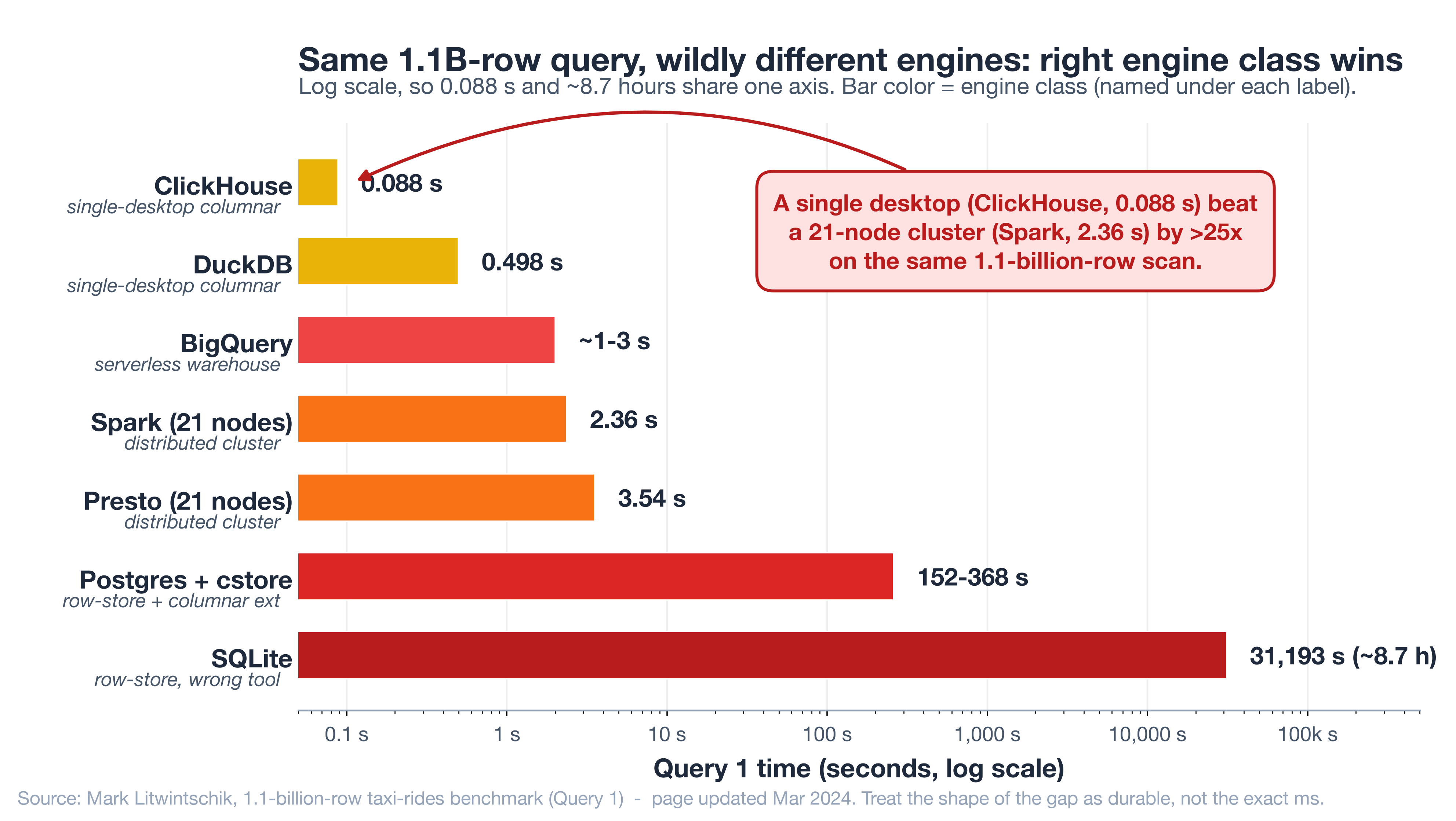
Same query, same 1.1B-row dataset, across engine classes. Source: Mark Litwintschik, 1.1 Billion Taxi Rides benchmarks, page updated March 2024.
Engine class 3: Distributed — horizontal scale, and the fan-out ceiling
When one node genuinely can’t hold the data or serve the writes, distributed engines spread the work across many. The mental model most people carry — more nodes, more speed — holds right up until it doesn’t, and knowing where that line sits is the difference between a defensible cluster and a single box with a network bill attached.
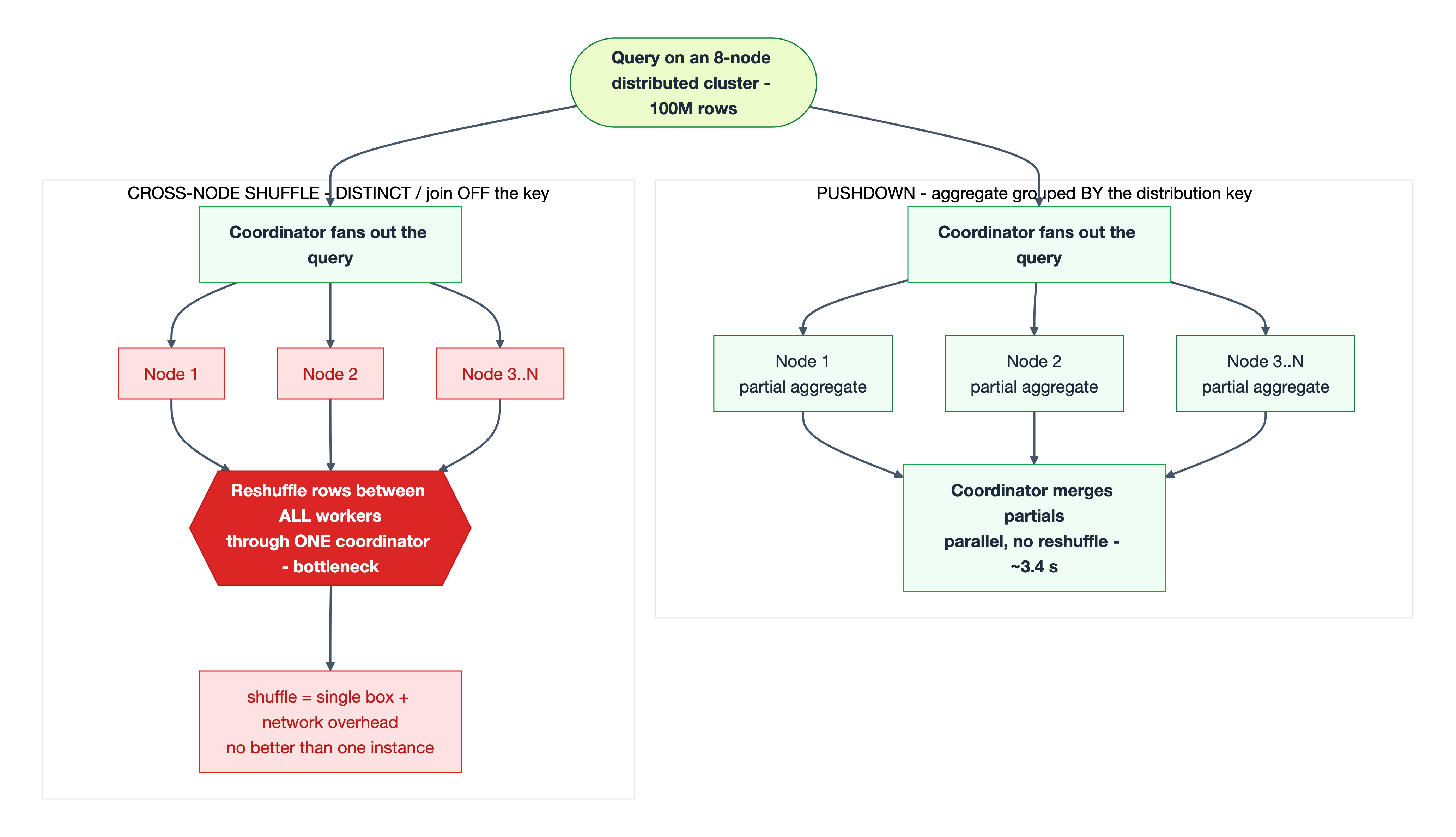
The line: does the query push down to the shards, or force a reshuffle? Distribute by tenant_id and group by tenant_id, and each node computes its slice while the coordinator stitches the results together. That’s pushdown, and it parallelizes beautifully. But the moment a query needs data spread across nodes — a count(DISTINCT) on a non-distribution column, or a join across the distribution boundary — the engine has to reshuffle rows between workers first. That shuffle is the ceiling.
The Citus benchmark puts numbers on it (100M rows, 8 nodes, 32 shards; PG 9.5.4, 2016 — again mechanism-illustrative). A plain count(*) across the cluster ran about 1.2s. A count(DISTINCT) on the distribution column, which pushes down, ran about 3.4s. On a non-distribution column it can’t push down, and pulling every row back to the coordinator is, in Nelson’s words, “really no better than counting on a single database instance … plus high network overhead.” An HLL approximate distinct ran 3.2–3.8s — the row-store’s approximation trick again, now buying a way around the shuffle. This generalizes well past Citus: in Spark the expensive stage is almost always the shuffle, and distributed query design is mostly the craft of keeping the hot queries pushed down.
So distributed isn’t a “scale” button. It’s a trade — horizontal capacity for query flexibility and operational complexity. Align your access pattern with the distribution key and it’s transformative. Keep needing cross-node data and you’ve bought nodes and network latency to arrive back at roughly single-box performance. That mismatch is its own crossover signal, and the one most likely to be discovered the hard way in production.
The memory / spill axis — the one most write-ups skip
Now the second axis, and the reason “just add an index” so often does nothing. A query can be on exactly the right engine class and still fall off a cliff, because its sorts and hash tables outgrew the memory the engine was allowed and spilled to disk. This is engine-independent: columnar and distributed engines build the same buffers and spill the same way when they overflow their limits. Postgres is just the easiest place to watch it, because its docs name the knob.
The spill cliff
At the default 4MB work_mem (PostgreSQL docs), a GROUP BY, DISTINCT, or ORDER BY that builds something larger switches from an in-memory hash or sort to an external merge that writes temp files to disk. The Citus benchmark shows the size of the drop (PG 9.5.4, 2016; mechanism unchanged per the current docs): at default work_mem, count(DISTINCT) on an integer column averaged 743ms, but on a text column 31,747ms — a ~43× gap — with Sort Method: external merge Disk in the plan. Give the operation enough work_mem to stay in RAM and the integer case drops to about 372ms as an in-memory HashAggregate. That in-RAM-versus-disk boundary is the axis. Stay on the right side and the query flies; cross it and it collapses.
This is exactly why indexing didn’t help the composite team. An index changes how you find rows; it does nothing for a GROUP BY/DISTINCT whose result set is too big for work_mem. The lever there is memory, or a smaller working set — not another index.
When to re-architect instead of tune
work_mem is allocated per operation per query, and the docs warn total usage “could be many times” that value under load, so raising it globally just trades a spill problem for an out-of-memory one. Past a point the honest move is structural. PostgreSQL’s partitioning guidance offers a clean rule: partition “when the size of the table [would] exceed the physical memory of the database server.” Pruning then skips whole partitions — but it isn’t free. The planner handles “up to a few thousand” partitions well only if pruning leaves few, since “each partition requires its metadata to be loaded into the local memory of each session that touches it.” Thousands of poorly-pruned partitions is its own problem.
One more trap: deep pagination
LIMIT ... OFFSET n gets slower the further you page. As Markus Winand explains in “No Offset”, the database “fetches and drops” all n preceding rows before returning the page, and results drift when rows are inserted between requests. A keyset (seek) query filters on the last-seen sort key instead and stays roughly constant-time however deep you go. Page latency that climbs with depth is a spill-adjacent signal, not a hardware one.
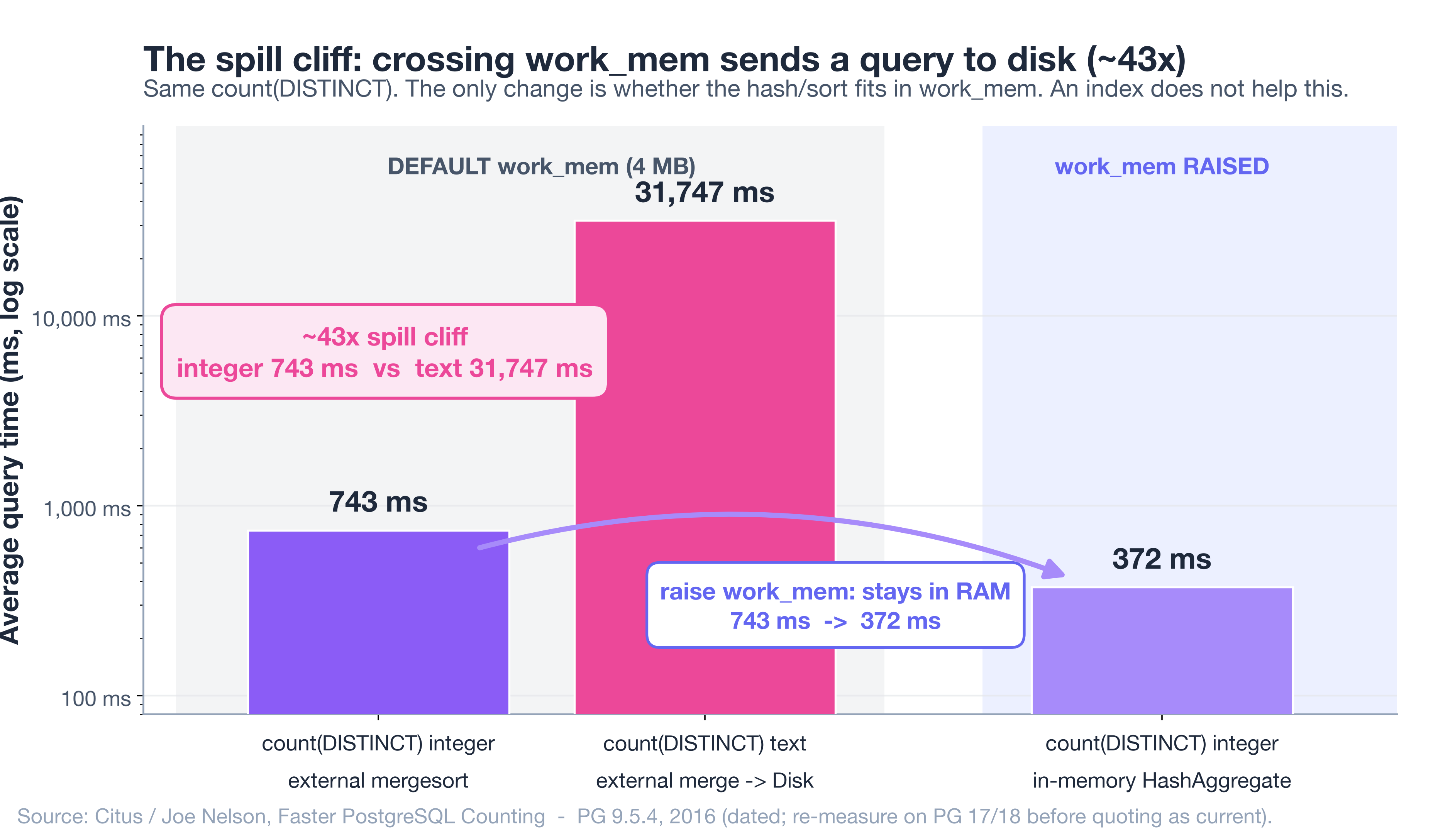
count(DISTINCT) at default vs raised work_mem. Source: Citus / Joe Nelson, PostgreSQL 9.5.4, 2016 — illustrative of the mechanism, not current figures.
The crossover-signal checklist: change engine class, don’t add another index
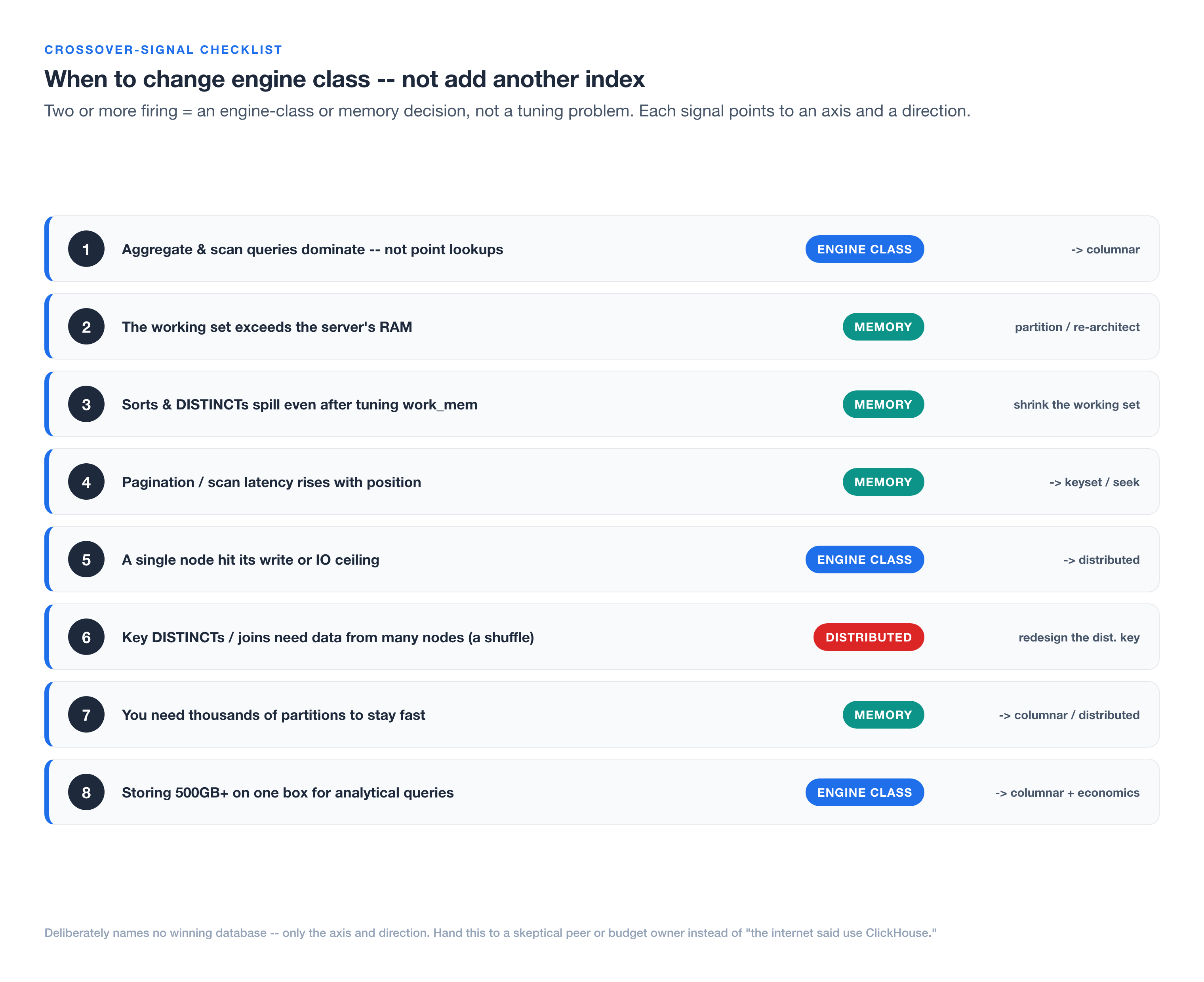
This is the piece worth saving. A framework’s job is to tell you when you’ve hit the boundary and it’s time to move on an axis instead of tuning further. Eight signals I watch for, each tied to the axis it moves. Two or more firing means you’re past tuning and into an engine-class or memory-budget decision.
- Scans and aggregates dominate the workload (not point lookups). → Engine class, toward columnar. The row-store aggregate cliff; indexing won’t fix an off-design pattern.
- The working set exceeds server RAM. → Memory. Postgres’s own partition threshold; partition, re-architect, or move to columnar/distributed.
- Sorts and
DISTINCTs keep spilling even after tuningwork_mem. → Memory. You’ve hit the ceiling of per-query memory; the working set is the problem. - Pagination or scan latency rises with position. → Memory/scan; switch to keyset/seek before switching engines.
- A single node has hit its write or IO ceiling. → Engine class, toward distributed. The one genuine “add nodes” signal.
- Key
DISTINCTs or joins need data from several nodes (a shuffle). → A warning on the distributed axis: without a distribution-key redesign, more nodes ≈ one box plus network. - You need thousands of partitions to stay fast. → Memory/metadata; the per-partition cost says a columnar or distributed store fits the data better.
- You’re keeping 500GB+ on one box for analytics. → Engine class plus economics; columnar compression and distributed storage costs start driving the decision.
What the list deliberately doesn’t do is name a winning database. Each signal points to an axis and a direction, because the right specific engine depends on your query shapes, your team’s ops maturity, and your budget. “Change engine class” is an architectural decision with a reason attached — something you can hand a skeptical peer or a budget owner instead of “the internet said use ClickHouse.”
Cost and economics for the decision-makers
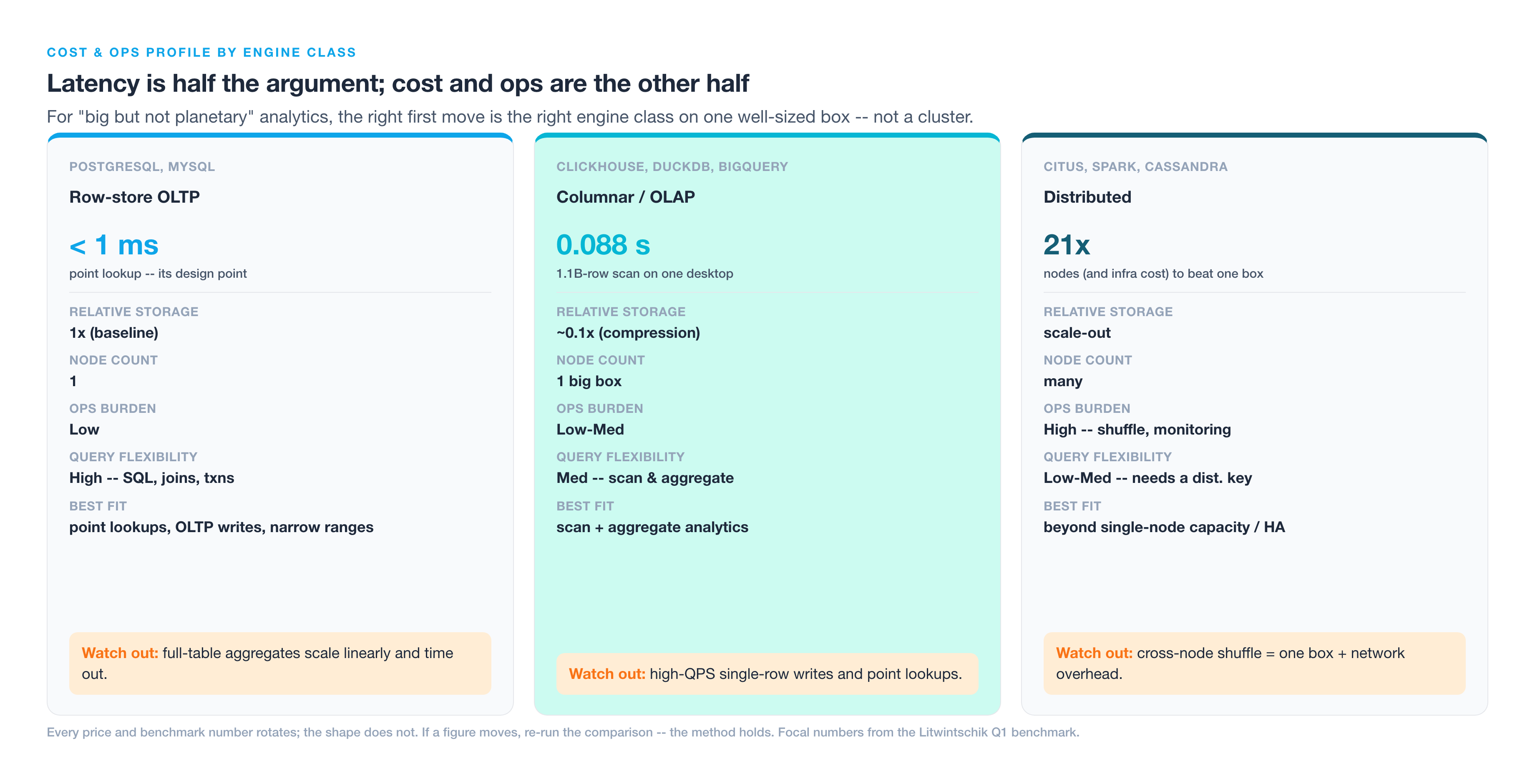
If you own the stack decision, latency is half the case; the half that gets budget approved is cost and defensibility. The benchmarks reframe cleanly as money.
A single big box can be cheaper and faster than a cluster. The Litwintschik result — one desktop-class node beating a 21-node cluster on a 1.1B-row scan — reads louder as a cost story than a speed one: 21 nodes carry ~21× the compute plus coordination, networking, and a standing ops burden, and still lose on this workload. For “big but not planetary” analytics, the first move is often the right engine class on one well-sized box, not a cluster. Distributed earns its cost when you truly exceed single-node capacity or need the availability.
Compression is a storage-cost lever. A columnar layout shrinks wide, repetitive data by a large multiple (measure it for your engines from ClickBench’s “Data Size” column — it varies by engine and codec), which is a recurring cut in bytes stored and, in a warehouse, fewer dollars per query scanned.
Per-query billing cuts both ways. A serverless warehouse (BigQuery ran 1–3s per query here) fits spiky, ad-hoc analytics where an idle cluster would bleed money, and fits badly for a high-frequency dashboard hammering one aggregate, where a right-sized columnar box wins on total cost.
Every price and benchmark here will rotate — pricing shifts, hardware moves the single-node ceiling, vendor benchmarks get re-run. Don’t anchor the decision to one dated figure. The framework doesn’t rotate: two axes, eight signals. If a price moves, re-run the comparison.
Build it yourself
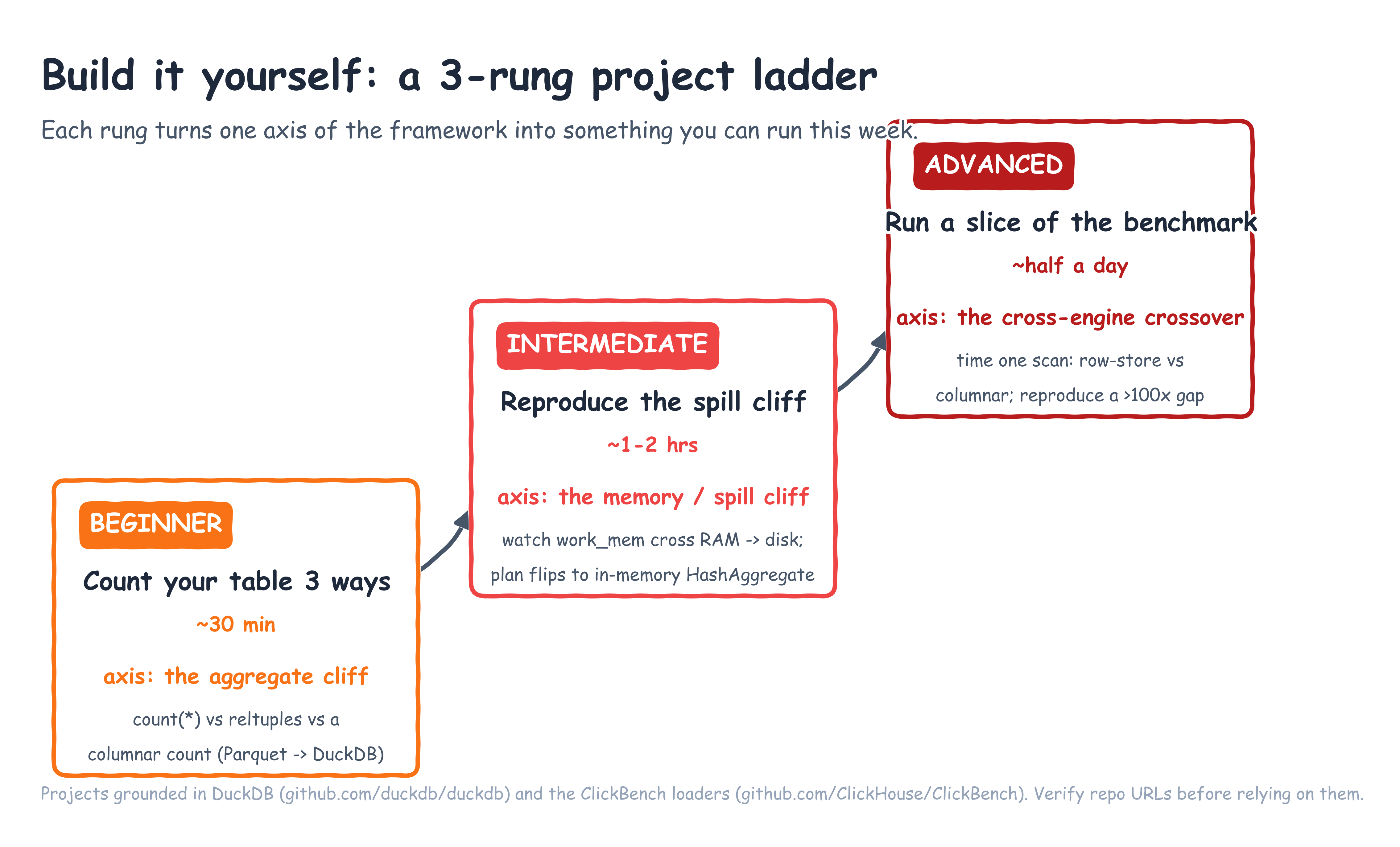
The framework is cheap until you feel it on your own data. Three projects, beginner to advanced. Each names a real tool (links verified reachable in 2026, but repos move — check before you lean on them).
Project 1 — Count your table three ways (~30 min). Feel the row-store aggregate cliff on real data. You’ll need a Postgres or MySQL table with 10M+ rows and DuckDB. Run EXPLAIN ANALYZE SELECT count(*) FROM your_table; and note the time and the Seq Scan; then SELECT reltuples::bigint FROM pg_class WHERE oid = 'schema.your_table'::regclass;; then get a slice into columnar form — export CSV (COPY your_table TO 'slice.csv' (FORMAT csv)) and load it into DuckDB, or read the table directly with pg_duckdb — and count(*) there. Done when you can state your own numbers for all three and point to the Seq Scan. Stretch: add GROUP BY day.
Project 2 — Reproduce the spill cliff (~1–2 hrs). Watch a query cross the RAM→disk boundary. You’ll need Postgres and a 1M+ row table with an integer and a text column (the NYC-taxi or ClickBench sets work). At default work_mem, run EXPLAIN ANALYZE SELECT count(DISTINCT int_col) FROM t; then the same on text_col, and confirm Sort Method: external merge Disk on the slow one. SET work_mem = '1GB';, re-run both. Done when you’ve captured your own before/after ratio and seen the plan flip to in-memory HashAggregate. Stretch: chart latency as you step work_mem from 4MB to 1GB and find your own cliff edge.
Project 3 — Run a slice of the 1.1B benchmark (~half a day). Reproduce the crossover on your hardware. You’ll need the same big table in a row-store and a columnar engine, plus the ClickBench loaders (60+ DBMS setup scripts) and Litwintschik’s posts for reference. Load an identical scan-aggregate table into each, time one representative query on both, and record the ratio and your hardware. Done when you reproduce a >100× gap — or can explain from the plans why yours differs. Stretch: add a distributed engine and build a query that forces a shuffle to find your own fan-out ceiling.
What to do Monday morning
The whole thing, compressed. When a query dies at scale, stop asking “which index?” and ask the two questions that decide it. Engine class: is the dominant shape point-lookups (row-store), scans and aggregates (columnar), or genuinely bigger than one node (distributed)? Memory budget: does the working set fit in RAM, or is it spilling? Then walk the eight signals; two or more means the move is on an axis, not another index. There’s no single answer to “how do I handle a billion rows” — the answer is a decision you can write down and defend.
So go run it. Take your biggest table this week and do Project 1: count(*), then reltuples, then a columnar count in DuckDB. Watch where the plan shows a Seq Scan and how far apart the three numbers land. Want the full crossover? The ClickBench repo has loaders for 60+ engines, so you can time the same scan on a row-store and a columnar engine side by side. Bring back your own numbers — the framework only lands once the cliff is yours.